PostGIS Mapping and Plotting
This guide covers the installation of Postgres/PostGIS and QGIS, importing Wake County’s GIS data, and creating a sample data plot using R. The Boundless Intro to PostGIS is an excellent guide to using PostGIS and I would highly recommend reading through it.
Installation and Loading/Checking Data
Install Postgres and the PostGIS extension and add a user for your login name:
sudo apt-get install postgis postgresql-9.3-postgis-2.1
sudo -u postgres createuser -d shawn
Create a database and add the PostGIS extension to it:
createdb wake
sudo -u postgres psql -d wake -c "CREATE EXTENSION postgis;"
WakeGIS provides GIS data for Wake County. Download the property file, extract it, and review the contents. The data is in Shapefile format, so we’ll need to figure out how to get it into Postgres. Loading Data is a quick overview of the process of loading arbitrary shapefiles. The tricky part is getting the correct Spatial Reference System Identifier (SRID) for the data, which uniquely identifies the projection system used to generate the coordinates for the geometric data. The .prj file included with the data has information about the projection used for the shape file. Examine the SRID table in postgres:
$ psql -d wake
psql (9.3.13)
Type "help" for help.

wake=> SELECT srid, srtext FROM spatial_ref_sys WHERE srtext LIKE '%North Carolina%';
The output is too long to show here, but SRID 2264 appears to be the closest to the description in the .prj file. With that knowledge, the data can be loaded into the database from the shape files (it can take a minute or two):
shp2pgsql -s 2264 properties_2016_07.shp properties wake > properties_2016_07.sql
psql -d wake -f properties_2016_07.sql | uniq -c
Loading from a file would normally print an entry for every insert. Piping to uniq -c will print a count for each unique line of text instead, creating a summary. There are about 350,000 separate property boundaries in Wake County:
2 SET
1 BEGIN
1 CREATE TABLE
1 ALTER TABLE
1                      addgeometrycolumn
1 ------------------------------------------------------------
1  public.properties.geom SRID:2264 TYPE:MULTIPOLYGON DIMS:2
1 (1 row)
1
349258 INSERT 0 1
1 COMMIT
The first thing that you may want to do with the property data is select a property based on a latitude/longitude from online maps. As it turns out, this is a little tricky. The data from Wake County is in NAD83 which looks nothing like latitude/longitude (WGS84). This query shows the computed center of Moore square in the “Extended Well Known Text” (EWKT) format that includes the SRID:
wake=> SELECT ST_AsEWKT(ST_Centroid(geom)) FROM properties WHERE propdesc='MOORE SQUARE';
                st_asewkt
------------------------------------------
SRID=2264;POINT(2108030.09758677 738098.650233197)
(1 row)
Note that the output point is not in the more-familiar latitude/longitude format. Here’s an example of selecting a property using a point (from the above coordinates). The ::geometry appended to a string casts text to a geometry that we can compare to entries in the property table:
wake=> SELECT propdesc FROM properties WHERE ST_Contains(geom, 'SRID=2264;POINT(2108030.09758677 738098.650233197)'::geometry);
   propdesc
--------------
 MOORE SQUARE
(1 row)
So now we need to figure out how to get the lat/long numbers into something that we can work with. We can work backwards by converting the NAD83 to WSG84 using ST_Transform to see what we get. Looking at OpenStreetMaps, the latitude and longitude for is in the URL (e.g. https://www.openstreetmap.org/export#map=19/35.77747/-78.63575) so we’ll expect to get approximately (35,-78):
wake=> SELECT ST_AsEWKT(ST_Transform('SRID=2264;POINT(2108030.09758677 738098.650233197)'::geometry, 4326));
                      st_asewkt
-----------------------------------------------------
 SRID=4326;POINT(-78.6357899299718 35.7774829946632)
(1 row)
Instead the point in (-78,35). Apparently the point data is (lon, lat), NOT (lat, lon)!!! So now that we can convert between systems and know the ordering to provide the data in, we can go look up arbitrary lat/lon information in OSM and query our parcels. If we use the lat/long from looking at the URL with the map over another square (https://www.openstreetmap.org/export#map=19/35.78023/-78.63922) we should get it back out:
wake=> SELECT propdesc FROM properties WHERE ST_Contains(geom, ST_Transform('SRID=4326;POINT(-78.63922 35.78023)'::geometry, 2264));
    propdesc
----------------
 CAPITOL SQUARE
(1 row)
Perfect! Now we can query an arbitrary neighborhood, parcel, etc. in the database using coordinates from online maps, GPS, etc.
Relating Data
So now we can download and add data that will contain interesting boundaries. There are census blocks/tracts, neighborhoods, etc.
unzip Wake_ZipCodes_2016_07.zip
shp2pgsql -s 2264 Wake_ZipCodes_2016_07.shp zips wake > Wake_ZipCodes_2016_07.sql
psql -d wake -f Wake_ZipCodes_2016_07.sqlpsql -d wake -f Wake_ZipCodes_2016_07.sql | uniq -c

unzip Wake_Census_2010.zip
shp2pgsql -s 2264 Wake_Tracts_2010.shp census_tracts wake > Wake_Tracts_2010.sql
shp2pgsql -s 2264 Wake_Blocks_2010.shp census_blocks wake > Wake_Blocks_2010.sql
shp2pgsql -s 2264 Wake_BlockGroup_2010.shp census_blockgroups wake > Wake_BlockGroup_2010.sql
psql -d wake -f Wake_Blocks_2010.sql | uniq -c
psql -d wake -f Wake_BlockGroup_2010.sql | uniq -c
psql -d wake -f Wake_Tracts_2010.sql | uniq -c

unzip Wake_Subdivisions_2016_07.zipunzip Wake_Subdivisions_2016_07.zip
shp2pgsql -s 2264 Wake_Subdivisions_2016_07.shp subdivisions wake > Wake_Subdivisions_2016_07.sql
psql -d wake -f Wake_Subdivisions_2016_07.sql | uniq -c
With all of those datasets installed we’re set to start joining on subdivisions to get interesting data out. Given the name of a neighborhood (I picked Westchester as an example), you can select all of the properties within it:
 SELECT sale_date, totsalpric, siteaddr
 FROM properties
 JOIN subdivisions ON ST_Within(properties.geom, subdivisions.geom)
 WHERE subdivisions.name = 'WESTCHESTER'
 ORDER BY sale_date DESC;
Visualizing with QGIS
We can also see the data visually by firing up QGIS. Install QGIS and optionally the Python support to enable plugins:
sudo apt-get install qgis python-qgis
Add a password to your Postgres user (ALTER USER shawn WITH PASSWORD 'password';) so that QGIS can connect on a network socket. Start up QGIS, navigate to the “Browser” tab and add a new Postgres server, using “localhost” as the hostname and “wake” as the database. To see the data in a given table, add a layer from the browser for that table.
Next create a view of the properties table that will be only the properties that we want to plot:
CREATE VIEW westchester
AS SELECT properties.gid, properties.geom
   FROM properties
   JOIN subdivisions ON ST_Within(properties.geom, subdivisions.geom)
   WHERE subdivisions.name = 'WESTCHESTER';
Now add the layer for the Westfield neighborhood itself. Since it’s only one data point without a join, we’ll use the QGIS query functionality to select it:
- Click the “Add PostGIS Layers” button to the left
- Connect to the database we added earlier
- Select the “subdivisions” table
- “Set Filter” and add the expression
"name" = 'WESTCHESTER', then test. It should return one row. - Add the layer
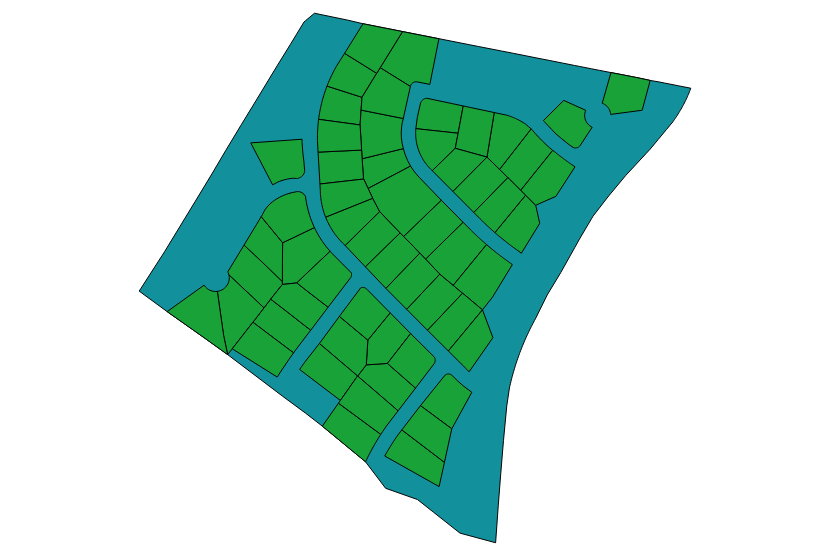
Now we can see the outline of this one neighborhood:

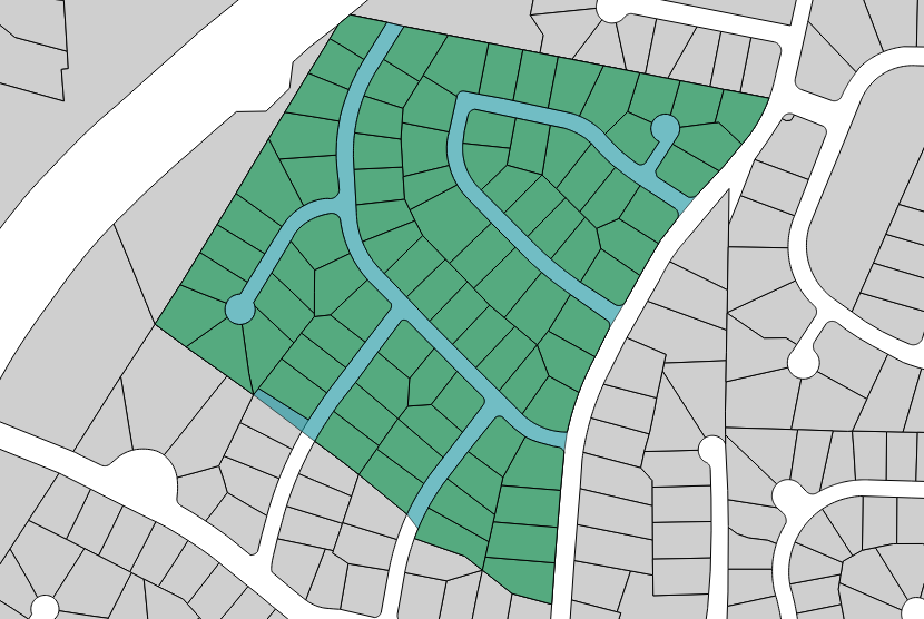
Add the layer for the Westchester houses from the browser tab:
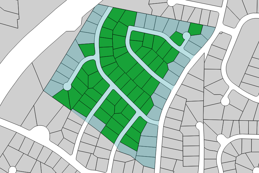
Oops, it looks like we don’t have all of the properties that we want using ST_Within! We can compare what we selected to what we should select by adding the whole properties data.
Add the properties layer, move the new layer to the bottom, and make the neighborhood layer more transparent:
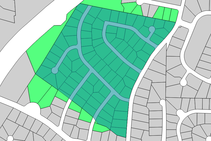
ST_Intersects as the join function is worse in the other direction:
We will clean this up by using the ST_Centroid function to compute the center of the property and checking whether that point is within the neighborhood. Unfortunately it looks like there are invalid shapes in the table:
wake=> SELECT prop.gid, prop.geom FROM properties AS prop JOIN subdivisions ON ST_Within(ST_Centroid(prop.geom), subdivisions.geom) WHERE subdivisions.name = 'WESTCHESTER';
ERROR:  First argument geometry could not be converted to GEOS: IllegalArgumentException: Invalid number of points in LinearRing found 3 - must be 0 or >= 4
But we can limit the data that it checks by checking the bounding box first using geom1 && geom2:
CREATE VIEW westchester_centroid
AS SELECT prop.gid, prop.geom
   FROM properties AS prop
   JOIN subdivisions ON prop.geom && subdivisions.geom
                    AND ST_Within(ST_Centroid(prop.geom), subdivisions.geom)
   WHERE subdivisions.name = 'WESTCHESTER';
Success!
Plotting Data
This isn’t GIS specific, but it’s still interesting to plot data from spatial queries. We will use R and ggplot to create a scatterplot with a best fit linear line. Install RStudio (I already have RStudio installed, so installation is outside of the scope of this guide).
Install a Postgres module (RPostgreSQL)and it’s dependencies:
sudo apt-get install libpq-dev
rstudio
> install.packages("RPostgreSQL")
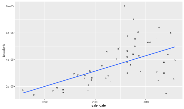
Then plot the data from the Westchester neighborhood, selecting the sale date (sale_date) and sale price (totsalpric). This is likely flawed since the sale date and price are per house rather than the entire sale history for every house, but it will do for a quick eyeball:
> library(RPostgreSQL)
> con <- dbConnect(PostgreSQL(), user="shawn", password="password", dbname="wake")
> out <- dbGetQuery(con, "SELECT sale_date, totsalpric, siteaddr FROM properties JOIN subdivisions ON properties.geom && subdivisions.geom AND ST_Within(ST_Centroid(properties.geom), subdivisions.geom) WHERE subdivisions.name = 'WESTCHESTER' AND totsalpric != 0 AND sale_date > '1981-01-01' ORDER BY sale_date DESC;")
> #plot it:
> library(ggplot2)
> ggplot(out, aes(sale_date, totsalpric)) + geom_point(shape=1) + geom_smooth(method=lm, se=FALSE)